A waterfall chart is a visual representation of a hierarchy in a vertical column. The waterfall charting method shows how work progresses during a period of time. It uses red lines to represent bad performance and green lines to represent good performance.

Have you ever gotten a data request that required a waterfall chart, how create waterfall chart in excel, how do i create a waterfall chart in excel template? If not, maybe you will soon. A waterfall chart is a great powerpoint slide that tells the story of how one thing affects another. It’s a real-world depiction of cause and effect — sort of like the graphic in this blog post.

How to build a waterfall chart in excel

A waterfall chart is a variation of the stacked bar chart. It is used to show the percentage contribution of individual values to the total. It is also known as a cumulative stacked bar chart or a stepped bar chart.

There are two ways you can create a waterfall chart in Excel: manually or using a template.

Create Waterfall Chart in Excel Manually

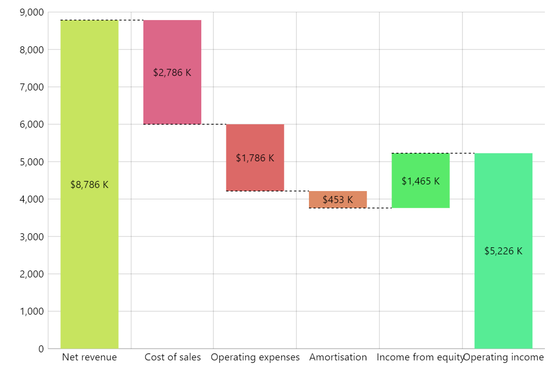
Waterfall charts are a pictorial representation of profit and loss over time. These charts are used to illustrate the breakdown of revenue and expenses over time, which can be useful for businesses to gain insight into how much money is coming in and going out.

Waterfall charts are not commonly used in Excel, but it’s possible to create them with some effort. This article will show you how to create a waterfall chart in Excel, along with some tips for formatting it.

The process for creating a waterfall chart in Excel involves four steps:

Create the chart itself by adding data to rows and columns in your spreadsheet. Add labels for each row or column that will eventually become part of the waterfall chart. Add an additional column or row above your data that will display totals at different points in time. Add a total row at the end of your worksheet that lists all totals from previous rows so they can be added up at once instead of being added manually every time they appear on screen.

In this tutorial, we will learn how to create a waterfall chart in Excel. A waterfall chart is a variation of a stacked bar chart. It has multiple rows for each item in the series.

Waterfall Charts are commonly used to show the break-up of expenses into various categories and sub-categories. For example, let’s say you have a budget of $200 for entertainment expenses, which consists of movies ($50), restaurants ($20), books and magazines ($30), and drinks at home ($70). The waterfall chart below shows how these expenses break up when viewed over time:

How to Create Waterfall Charts in Excel

Creating a waterfall chart in Excel is very easy. All you have to do is follow these simple steps:

Select the data range that you want to convert into a waterfall chart. Right-click on any cell within this range and select “Insert” from the context menu (or press CTRL + M). This will open the “Choose Chart Type” dialog box where you can select “Waterfall” from under “Stacked Bar” category:

Once done, click on OK button and see how your waterfall chart looks like:

Waterfall charts are one of the most popular types of charts and can be quite effective at communicating complex data. In this post, we’ll walk through how to create a waterfall chart in Excel.

How to Create a Waterfall Chart in Excel

To get started, you need to have some data that you want to put into your waterfall chart. Your data should be arranged as follows:

The first column should contain the values in your data set (e.g., sales figures for each month)

The second column should contain the totals for each value (e.g., total sales for each month). If there are multiple rows for each month, then this column will show the sum of those rows

The third column should contain percentages or other measures of relative size (e.g., percentages of total sales). If there are multiple rows for each month, then this column will show the percentage increase/decrease from previous months

Waterfall charts are a great way to show how much money is being spent and where it’s going. Waterfall charts are also called “Balanced Scorecards”, but they’re basically the same thing.

Waterfall charts are basically a list of numbers that show how much money you’ve made or lost in each area of your business or organization. They can be used for anything from personal budgets to corporate finances.

Here’s an example:

You can use a waterfall chart to see how you’re spending your time, money, and energy on different projects. For example, if you have three main projects that you’re working on right now, it might look something like this:

If you want to create a waterfall chart in Excel, follow these steps:

1) Create a table in your spreadsheet with four columns: “Name”, “Activity”, “Cost”, and “Profit”.2) In the first row of this table, enter the names of each activity you want to track (for example, “Marketing”, “Development”, etc.).3) In each row after that, enter the amount of money spent on each activity in its respective column (for example, $50 for marketing).4)

How create waterfall chart in excel

A waterfall chart is a graphical representation of the cumulative effect of adding successive values. It is usually used to display data such as annual sales, profits and net income over time.

Waterfall charts are one of the most common types of charts used in accounting and finance. They are often used to show the profit or loss at various stages of an investment or project.

To create a waterfall chart in Excel, you need to use the following steps:

Step 1: Select a cell, then click Insert tab > Table > Table Styles > Gridlines > None.

Step 2: Select another cell, then click Home tab > Alignment group > Horizontal Alignment > Center.

Step 3: Select another cell, then click Home tab > Number group > Number Format button > Custom from the drop-down menu. In the Type box, type 0% and click OK button to apply this formatting style for all numbers in your worksheet range except for zeroes that represent percentages on your waterfall chart template.

Step 4: Select another cell and type =0 into it; then press CTRL+SHIFT+ENTER keys together (or right-click on this cell and select Copy Special option).

How to create a waterfall chart in Excel?

A waterfall chart is a bar chart that is used to show the breakdown of an amount into its components. It’s a type of pie chart with multiple slices that represent the values added up from each category.

Waterfall charts are good for showing how an initial value is broken down into smaller parts, but they don’t work well for comparing two or more values in a single graph.

Creating a Basic Waterfall Chart

To create a basic waterfall chart in Excel, use the Table feature and create a column for each component of your total. Then use conditional formatting to color each column based on whether it’s positive or negative (yellow or blue). Next, drag the blue columns down until they’re hidden by the yellow ones, creating a zigzag pattern. Finally, hide all but one of the blue columns so that only one blue column remains visible.

How to Create a Waterfall Chart in Excel

In this Article:Making a Waterfall Chart in Microsoft ExcelCreating a Waterfall Chart in PowerPointCommunity Q&A

A waterfall chart is a type of chart that shows how money will be allocated. They are typically used in business and finance, but can also be used for personal budgets or savings goals. To create a waterfall chart, you must first create an Excel spreadsheet with rows and columns labeled with the names of your categories or expenses. Then, you will use formulas to show how much money will be allocated to each category or expense. Finally, you can add lines to your spreadsheet to create the waterfall effect on your chart.

Method 1:Make a Waterfall Chart with Microsoft ExcelThe first method is to make a waterfall chart using Microsoft Excel by following these steps:Step 1: Create an empty spreadsheet with rows and columns labeled with the names of your categories or expenses. This should look like this:

How to Create a Waterfall Chart in Excel

A waterfall chart is a type of chart that’s best used to show the breakdown of costs for different stages of a project or process. This type of chart can be created in Microsoft Excel, but you’ll need to install a separate add-in for it. Fortunately, there are plenty of free versions available online.

1. Open Microsoft Excel and select the “Insert” tab at the top of your screen.

2. Click on “Charts” from the menu on the left side of your screen and then select “Waterfall”.

3. Click on “Create Waterfall Chart” and then enter your data into the relevant cells in your spreadsheet.

You can create a waterfall chart in Excel by using the waterfall chart template. However, if you don’t have access to the template, you can still create a waterfall chart manually.

Here’s how it works:

1) Open up your Excel sheet and insert a new column in the data series for each category. If your categories are “Sales,” “Expenses,” etc., then you will need to add another column for each one of these categories.

2) Then, add a new row below each of these new columns. In this row, type in the formula =IF(NOW()<>“”,””,IF(A2